POTENTIAL PAYBACK PERIOD (PPP) : A NEW METRIC FOR STOCK EVALUATION TO ADDRESS THE SHORTCOMINGS OF THE TRADITIONAL PRICE-EARNINGS (PE) RATIO
ABSTRACT
Though the Price-Earnings (PE) Ratio offers simplicity in assessing stock attractiveness, it fails to explicitly account for fundamental variables such as the earnings growth rate and interest rate, which particularly affects the evaluations of high-growth stocks. While attempts, such as the Price-Earnings to Growth (PEG) ratio offer improvements on the PE Ratio, they remain empirical (being just a rule of thumb). Therefore, the Potential Payback Period (PPP) is proposed as a new metric for stock evaluation, with the objective of addressing the limitations of the PE Ratio. PPP rigorously integrates earnings growth through a mathematical formula, incorporates interest rates for discounting future earnings, and defines the time needed to equalise stock prices with future earnings. This synthetic, forward-looking metric, which can be called "Dynamic PE Ratio", allows for meaningful stock comparisons, especially in cases where the traditional PE Ratio is deficient, such as start-ups or companies with erratic earnings. PPP's logical coherence, translated into meaningful figures, makes it a valuable tool, demonstrating the financial market's rationality and providing a dynamic approach to stock evaluation.
KEY WORDS
Stock evaluation, Potential Payback Period (PPP), price-earnings (PE) ratio, earnings growth rate, interest rate, Price-Earnings to Growth (PEG) ratio, financial market, synthetic metric, dynamic perspective, high-growth stocks, start-ups.
INTRODUCING THE POTENTIAL PAYBACK PERIOD (PPP): A NEW METRIC FOR STOCK EVALUATION TO ADDRESS THE SHORTCOMINGS OF THE PRICE-EARNINGS (PE) RATIO
Initially popularized by Benjamin Graham, who is widely known as the "father of value
investing" and wrote the discipline’s founding text, “Security Analysis” in 1934, the Price-Earnings (PE)
Ratio remains the cornerstone metric for stock investors.
This measure has the merit of simplicity, because it is obtained through a simple division of stock prices by the
corresponding earnings per share.
However, although it is only meant to offer a quick glance at the relative “attractiveness” or “expensiveness” of
a stock, the PE Ratio soon reveals its shortcomings or operational limitations as a management tool.
Specifically, there are two fundamental variables in stock evaluation. The PE Ratio does not explicitly consider
the earnings growth rate and interest rate, whose variations strongly and daily influence stock prices.
The questionable applicability of the PE Ratio to high-growth stocks
The first shortcoming of the PE Ratio is its inability to properly assess the value of high-growth stocks.
Why do high-growth stocks with "prohibitive" PE Ratios continue to outperform the markets?
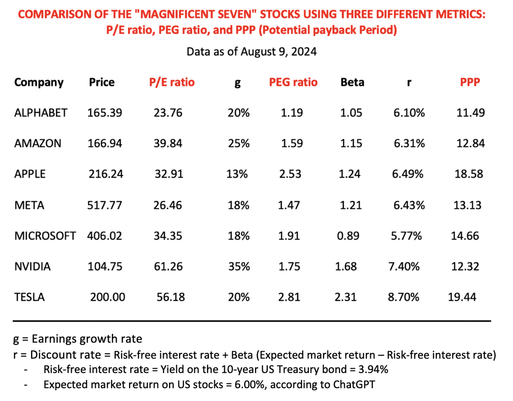
For instance, a group of US stocks (Alphabet, Amazon, Apple, Meta, Microsoft, Nvidia and Tesla), known as the
“Seven Magnificent”, are all relatively recently founded and have exhibited exponential growth in sales and
profit, coupled with exponential increases in their share prices. Such valuations have led to PE Ratios which,
according to traditional criteria, appear to be extremely high. Nevertheless, these high-growth stocks have
outperformed the market over the last ten years or more.
Intuitively, we accept the idea of relatively high PE Ratios for companies experiencing rapid growth. However, how
high is justified and where is the limit? Can we still buy these shares, and at what prices should they be sold?
The PE Ratio seems ill-suited to measure the "attractiveness” or "expensiveness" of a stock because it does not
explicitly take earnings growth into account. We empirically observe a correlation between the PE Ratio and
expected earnings growth rate, but there is no proportionality between the two. Therefore, conducting
well-established evaluations and comparisons is difficult.
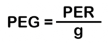
The Price-Earnings to Growth (PEG) Ratio is the first metric that adjusts the PE
Ratio
based on the earnings growth rate, but it is just rule of thumb.
The PEG Ratio is considered a convenient approximation and is simply the result of dividing the PE Ratio by the
earnings growth rate. If the PE Ratio is symbolised by “PER” and the earnings growth rate by “g”, then,
 According to Wikipedia, the PEG concept was originally developed by
Mario Farina, who discussed it in his 1969
book, “A Beginner's Guide to Successful Investing in the Stock Market”. It was later popularised by Peter Lynch,
who stated in his 1989 book, “One Up on Wall Street”, that "The PE Ratio of any company that is fairly priced will
equal its growth rate”, meaning that the PEG Ratio of a fairly valued company will be equal to one. This implies
that any stock with a PEG Ratio above one would be considered “overvalued”.
As an equity valuation tool, the PEG Ratio is believed to enhance the PE Ratio because it provides a more complete
picture by introducing expected earnings growth into the calculation. However, the way earnings growth rate “g” is
factored in to obtain the PEG Ratio (just by dividing the PE Ratio by “g”) and the way the result of the division
is interpreted (with the figure “1” being the threshold above which a stock would be considered relatively
“overvalued”) show that the PEG Ratio essentially rests on a rule of thumb. Such an empirical and approximative
method may occasionally be useful, but has clear limitations, because it lacks a rigorous theoretical foundation
and, therefore, cannot be applied in all circumstances.
Origin of the Potential Payback Period (PPP)
The concept of PPP for stock evaluation is derived from the well-known "payback period" for investment selection
in corporate finance. I
first exposed it in a series of articles in the French-language review, Analyse Financière, in the 1980s. The
title of the first article (second quarter 1984) was "Le PER, un instrument mal adapté à la gestion mondiale des
portefeuilles. Comment remédier à ses lacunes” (The PE Ratio, an instrument ill-suited for global portfolio
management. How can we remedy these shortcomings)? The approach was subsequently explained in the reference book,
"Finance
d'Entreprise" (Corporate Finance), by Pierre Vernimmen, a professor at HEC, the most prestigious business
school in France.
The PPP is a new synthetic metric that incorporates earnings growth more
rigorously.
A stock’s Potential Payback Period (PPP) is defined as the precise amount of time necessary to equalise its
current price with the sum of future earnings per share after considering their growth rate “g”. Through a
slightly
more complex formula than that of the PEG Ratio, the PPP moves from an empirical and approximate approach to
mathematical logic and precision.
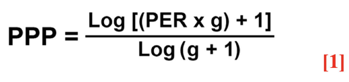
The following formula is used:
According to Wikipedia, the PEG concept was originally developed by
Mario Farina, who discussed it in his 1969
book, “A Beginner's Guide to Successful Investing in the Stock Market”. It was later popularised by Peter Lynch,
who stated in his 1989 book, “One Up on Wall Street”, that "The PE Ratio of any company that is fairly priced will
equal its growth rate”, meaning that the PEG Ratio of a fairly valued company will be equal to one. This implies
that any stock with a PEG Ratio above one would be considered “overvalued”.
As an equity valuation tool, the PEG Ratio is believed to enhance the PE Ratio because it provides a more complete
picture by introducing expected earnings growth into the calculation. However, the way earnings growth rate “g” is
factored in to obtain the PEG Ratio (just by dividing the PE Ratio by “g”) and the way the result of the division
is interpreted (with the figure “1” being the threshold above which a stock would be considered relatively
“overvalued”) show that the PEG Ratio essentially rests on a rule of thumb. Such an empirical and approximative
method may occasionally be useful, but has clear limitations, because it lacks a rigorous theoretical foundation
and, therefore, cannot be applied in all circumstances.
Origin of the Potential Payback Period (PPP)
The concept of PPP for stock evaluation is derived from the well-known "payback period" for investment selection
in corporate finance. I
first exposed it in a series of articles in the French-language review, Analyse Financière, in the 1980s. The
title of the first article (second quarter 1984) was "Le PER, un instrument mal adapté à la gestion mondiale des
portefeuilles. Comment remédier à ses lacunes” (The PE Ratio, an instrument ill-suited for global portfolio
management. How can we remedy these shortcomings)? The approach was subsequently explained in the reference book,
"Finance
d'Entreprise" (Corporate Finance), by Pierre Vernimmen, a professor at HEC, the most prestigious business
school in France.
The PPP is a new synthetic metric that incorporates earnings growth more
rigorously.
A stock’s Potential Payback Period (PPP) is defined as the precise amount of time necessary to equalise its
current price with the sum of future earnings per share after considering their growth rate “g”. Through a
slightly
more complex formula than that of the PEG Ratio, the PPP moves from an empirical and approximate approach to
mathematical logic and precision.
The following formula is used:
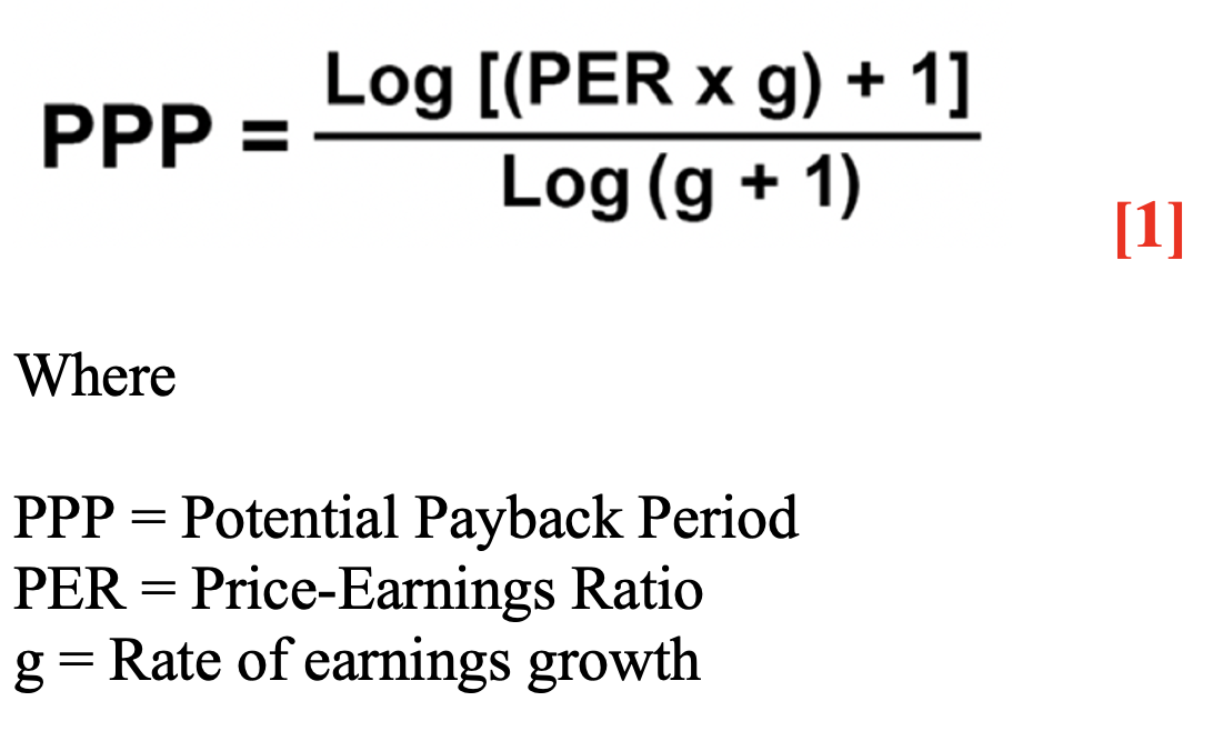 In the above PPP formula, "g" is the same earnings growth rate as that in the PEG formula:
Mathematical demonstration
The formula for the Potential Payback Period (PPP) for stock valuation is based on the sum of the first n terms of
a geometric sequence.
Consider the geometric progression: E0 , E0q , E0q2,
E0q3, ………… E0qn-1
Let’s the sum of n terms be P, the first term be E0 and the common ratio of geometric progression be q.
Then P = E0 + E0q + E0q2 + E0q3 + ……. +
E0qn-1 [A]
Multiply both sides of P by q, we obtain:
Pq = E0q + E0q2 + E0q3 + ……. + E0q [B]
Subtracting [B] from [A], obtain:
Pq - P = (E0q + E0q2 + E0q3 + … +
E0qn) – (E0 + E0q + E0q2 +
E0q3 + ……. + E0qn-1)
Pq - P = E0qn – E0
P (q – 1) = E0 (qn – 1)
P = E0 (qn – 1) / (q – 1)
Hence the sum of n terms of the geometric sequence is
P = E0 (qn – 1) / (q – 1)
P/E0 = (qn – 1) / (q – 1)
Now, we calculate n, which is the Potential Payback Period (PPP), and P is the current share price.
E0 is earnings per share in the current year.
P/E0 is the price–earnings ratio (PER), which we name X.
X = (qn – 1) / (q – 1)
qn – 1 = X (q – 1)
qn = X (q – 1) + 1
Log qn = Log [X (q – 1) + 1]
n Log q = Log [X (q – 1) + 1]
n = Log [X (q – 1) + 1] / Log q [C]
In our sequence of future earnings per share, if g is the annual earnings growth rate, then the common ratio q of
geometric progression is q = 1 + g, based on the compound interest formula.
On the right side of equation [C], (q – 1) = 1 + g – 1 = g.
Noting that n is the Potential Payback Period (PPP), X is the PE Ratio or PER, q – 1 = g
and q = g + 1, we derive, from [C]
By adjusting the PE Ratio to rigorously incorporate earnings growth, PPP allows for more meaningful stock
comparisons.
PPP is viewed in the same way as the PE Ratio, meaning that the smaller the value of the metric, the more
attractive the stock, all else being the same.
Variation of PPP with PE Ratio
The higher the earnings growth rate “g”, the shorter the PPP, which varies with respect to the PE Ratio in a
pattern as shown in the following graph.
In the above PPP formula, "g" is the same earnings growth rate as that in the PEG formula:
Mathematical demonstration
The formula for the Potential Payback Period (PPP) for stock valuation is based on the sum of the first n terms of
a geometric sequence.
Consider the geometric progression: E0 , E0q , E0q2,
E0q3, ………… E0qn-1
Let’s the sum of n terms be P, the first term be E0 and the common ratio of geometric progression be q.
Then P = E0 + E0q + E0q2 + E0q3 + ……. +
E0qn-1 [A]
Multiply both sides of P by q, we obtain:
Pq = E0q + E0q2 + E0q3 + ……. + E0q [B]
Subtracting [B] from [A], obtain:
Pq - P = (E0q + E0q2 + E0q3 + … +
E0qn) – (E0 + E0q + E0q2 +
E0q3 + ……. + E0qn-1)
Pq - P = E0qn – E0
P (q – 1) = E0 (qn – 1)
P = E0 (qn – 1) / (q – 1)
Hence the sum of n terms of the geometric sequence is
P = E0 (qn – 1) / (q – 1)
P/E0 = (qn – 1) / (q – 1)
Now, we calculate n, which is the Potential Payback Period (PPP), and P is the current share price.
E0 is earnings per share in the current year.
P/E0 is the price–earnings ratio (PER), which we name X.
X = (qn – 1) / (q – 1)
qn – 1 = X (q – 1)
qn = X (q – 1) + 1
Log qn = Log [X (q – 1) + 1]
n Log q = Log [X (q – 1) + 1]
n = Log [X (q – 1) + 1] / Log q [C]
In our sequence of future earnings per share, if g is the annual earnings growth rate, then the common ratio q of
geometric progression is q = 1 + g, based on the compound interest formula.
On the right side of equation [C], (q – 1) = 1 + g – 1 = g.
Noting that n is the Potential Payback Period (PPP), X is the PE Ratio or PER, q – 1 = g
and q = g + 1, we derive, from [C]
By adjusting the PE Ratio to rigorously incorporate earnings growth, PPP allows for more meaningful stock
comparisons.
PPP is viewed in the same way as the PE Ratio, meaning that the smaller the value of the metric, the more
attractive the stock, all else being the same.
Variation of PPP with PE Ratio
The higher the earnings growth rate “g”, the shorter the PPP, which varies with respect to the PE Ratio in a
pattern as shown in the following graph.
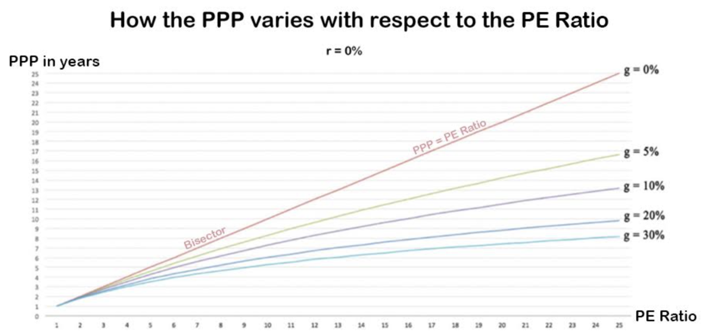 Graph : Variation of PPP with PE Ratio
When g = r = 0% (no profit growth, no inflation and no discounting requirement), PPP = PE Ratio. The curves of PPP
and
PE Ratio overlap and
correspond to the bisector.
As we will see later on, the same case where PPP = PE Ratio occurs whenever the nominal profit growth rate "g" is
equal
to
their
discount rate "r", that is when profits remain constant in present value. But these cases where PPP and PE Ratio
overlap are exceptional.
In the general case where "g" is different from "r" (g ≠ r), the curve of PPP falls below the bisector (PPP < PE
Ratio) when the profit growth rate "g" is higher than the discount rate "r" (g> r). PPP decreases more rapidly
relative
to PE Ratio as the profit growth rate "g" accelerates (from 0% to 30% per year in our example).
The PE Ratio is a special case of PPP, when there is no growth in earnings (and no discounting requirement).
As explained in an Investopedia
article entitled, “What Is the Price-to-Earnings (P/E) Ratio?”, “Simply put, a PE ratio of
15
would mean that the current market value of the company is equal to 15 times its annual earnings. Put
literally,
if you were to hypothetically buy 100% of the company’s shares, it would take 15 years for you to earn back
your
initial investment through the company’s ongoing profits, assuming the company never grew.” In this specific
case, g = 0% and PPP = P/E Ratio, as represented by the bisector in the graph above.
Because we must reject the unrealistic “0 growth” assumption, we have to factor in the earnings growth rate
“g”
as in PPP formula [1].
For example, if g = 8 (percent per year), the PPP would amount to 10.24 (down from 15
if g = 0). Instant calculations of the PPP can be performed at
https://stockinternalrateofreturn.com/instant_calculations.html
PPP’s sensitivity to the earnings growth rate, "g"
The stock market is highly sensitive to changes in expected earnings growth rates. It is not the growth rate
or
speed itself (concept of "first derivative" in physics), but its acceleration or deceleration (concept of
"second derivative") which matters the most.
This explains why stock prices can be sensitive to quarterly earnings revisions, which, through extrapolation,
can result in revisions in earnings growth rates over a period well beyond the quarters in question.
Any new earnings growth rate immediately and automatically modifies the PPP level, resulting in stock price
adjustments.
In any case, we must remember that the reliability and precision of any evaluation model, regardless of how
relevant it may be, depend on the reliability and precision of the data. For the PPP, the most sensitive data
is
"g", the estimated earnings growth rate for the next two to three years (tacitly and temporarily extrapolated
beyond), which has to be updated according to the most relevant and recent information. The same remark
applies
to the "g" used to calculate the PEG Ratio.
Incorporation of the interest rate "r" in the PPP
Furthermore, in order to take into account inflation and/or an opportunity cost for a stock investor, future
earnings must be discounted to their present values using a long-term risk-free interest rate, which we call
"r", as the discount rate.
With the introduction of the interest rate, "r", and based on the discount rate formula, the above-mentioned
sequence of future earnings per share becomes a geometric progression with (1 + g) / (1 + r) as common ratio.
In the previous demonstration of formula [1], we reached the point where
n = Log [X (q – 1) + 1] / Log q [C]
where n is the Potential Payback Period (PPP), X is the PE Ratio or PER, and q is the common ratio of the
geometric sequence of future earnings per share.
Now we have q = (1 + g) / (1 + r)
On the right side of equation [C], (q – 1) can be developed as follows:
(q – 1) = [(1 + g) / (1 + r)] – [(1 + r) / (1 + r)] = (g – r) / (1 + r)
Then,
n = Log [PER x [(g – r) / (1 + r )] + 1] / Log [(1 + g) / (1 + r)]
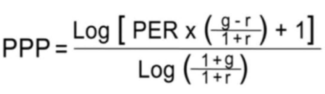
Finally here is the formula for PPP after the introduction of interest rate "r":
Graph : Variation of PPP with PE Ratio
When g = r = 0% (no profit growth, no inflation and no discounting requirement), PPP = PE Ratio. The curves of PPP
and
PE Ratio overlap and
correspond to the bisector.
As we will see later on, the same case where PPP = PE Ratio occurs whenever the nominal profit growth rate "g" is
equal
to
their
discount rate "r", that is when profits remain constant in present value. But these cases where PPP and PE Ratio
overlap are exceptional.
In the general case where "g" is different from "r" (g ≠ r), the curve of PPP falls below the bisector (PPP < PE
Ratio) when the profit growth rate "g" is higher than the discount rate "r" (g> r). PPP decreases more rapidly
relative
to PE Ratio as the profit growth rate "g" accelerates (from 0% to 30% per year in our example).
The PE Ratio is a special case of PPP, when there is no growth in earnings (and no discounting requirement).
As explained in an Investopedia
article entitled, “What Is the Price-to-Earnings (P/E) Ratio?”, “Simply put, a PE ratio of
15
would mean that the current market value of the company is equal to 15 times its annual earnings. Put
literally,
if you were to hypothetically buy 100% of the company’s shares, it would take 15 years for you to earn back
your
initial investment through the company’s ongoing profits, assuming the company never grew.” In this specific
case, g = 0% and PPP = P/E Ratio, as represented by the bisector in the graph above.
Because we must reject the unrealistic “0 growth” assumption, we have to factor in the earnings growth rate
“g”
as in PPP formula [1].
For example, if g = 8 (percent per year), the PPP would amount to 10.24 (down from 15
if g = 0). Instant calculations of the PPP can be performed at
https://stockinternalrateofreturn.com/instant_calculations.html
PPP’s sensitivity to the earnings growth rate, "g"
The stock market is highly sensitive to changes in expected earnings growth rates. It is not the growth rate
or
speed itself (concept of "first derivative" in physics), but its acceleration or deceleration (concept of
"second derivative") which matters the most.
This explains why stock prices can be sensitive to quarterly earnings revisions, which, through extrapolation,
can result in revisions in earnings growth rates over a period well beyond the quarters in question.
Any new earnings growth rate immediately and automatically modifies the PPP level, resulting in stock price
adjustments.
In any case, we must remember that the reliability and precision of any evaluation model, regardless of how
relevant it may be, depend on the reliability and precision of the data. For the PPP, the most sensitive data
is
"g", the estimated earnings growth rate for the next two to three years (tacitly and temporarily extrapolated
beyond), which has to be updated according to the most relevant and recent information. The same remark
applies
to the "g" used to calculate the PEG Ratio.
Incorporation of the interest rate "r" in the PPP
Furthermore, in order to take into account inflation and/or an opportunity cost for a stock investor, future
earnings must be discounted to their present values using a long-term risk-free interest rate, which we call
"r", as the discount rate.
With the introduction of the interest rate, "r", and based on the discount rate formula, the above-mentioned
sequence of future earnings per share becomes a geometric progression with (1 + g) / (1 + r) as common ratio.
In the previous demonstration of formula [1], we reached the point where
n = Log [X (q – 1) + 1] / Log q [C]
where n is the Potential Payback Period (PPP), X is the PE Ratio or PER, and q is the common ratio of the
geometric sequence of future earnings per share.
Now we have q = (1 + g) / (1 + r)
On the right side of equation [C], (q – 1) can be developed as follows:
(q – 1) = [(1 + g) / (1 + r)] – [(1 + r) / (1 + r)] = (g – r) / (1 + r)
Then,
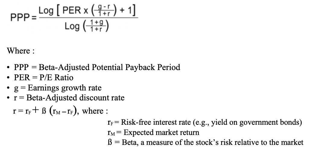
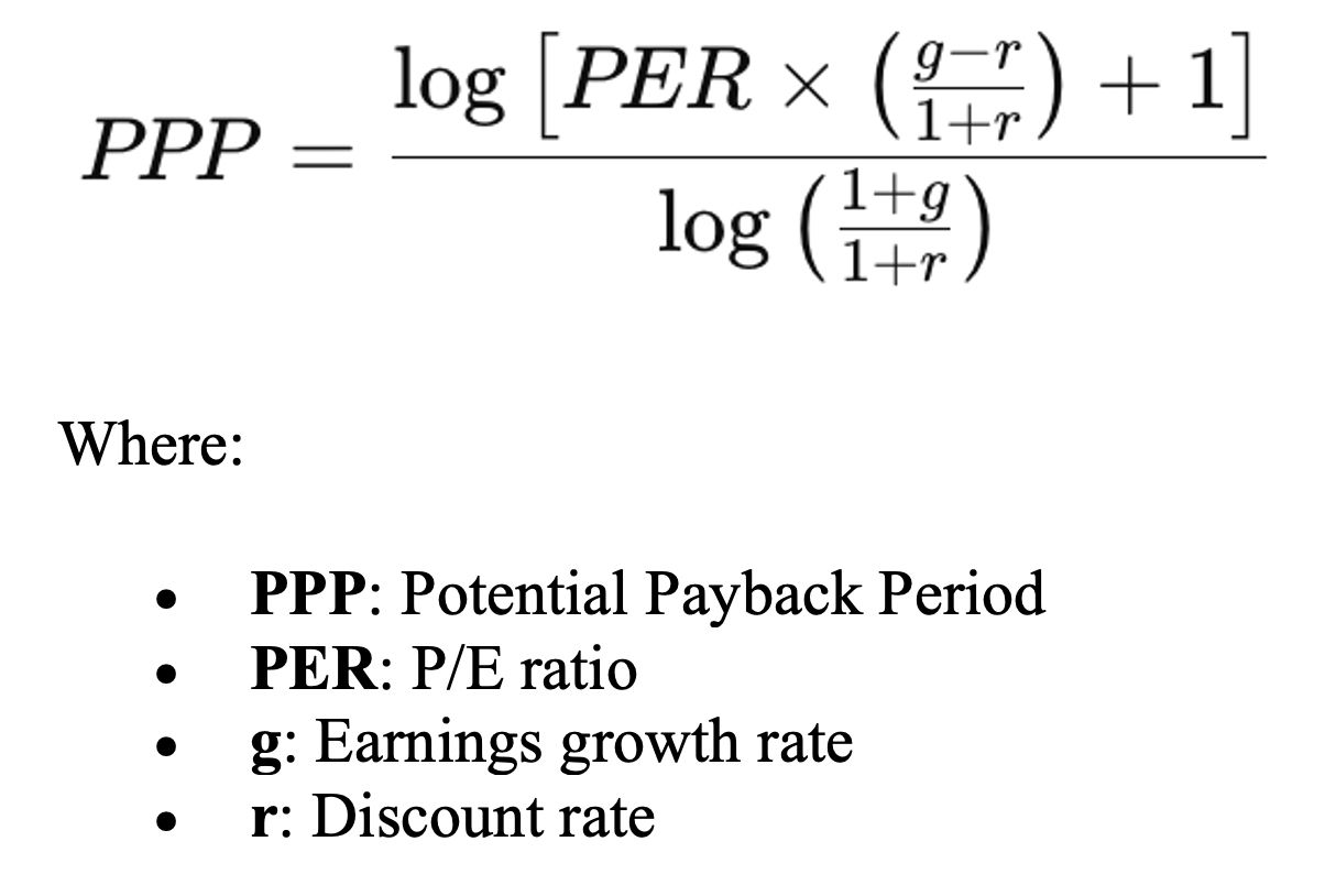
n = Log [PER x [(g – r) / (1 + r )] + 1] / Log [(1 + g) / (1 + r)]
Finally here is the formula for PPP after the introduction of interest rate "r":
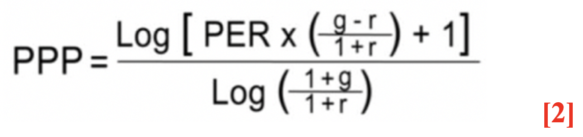 Therefore, by introducing an interest rate to discount future earnings, the Potential Payback Period (PPP)
transforms from
Therefore, by introducing an interest rate to discount future earnings, the Potential Payback Period (PPP)
transforms from
 to
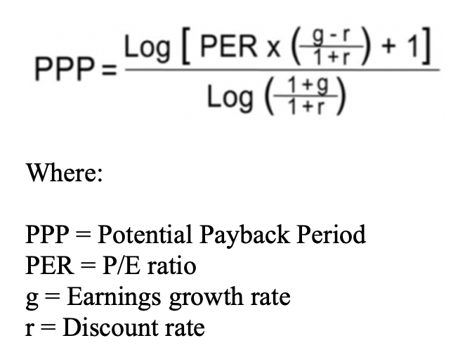
Where
PPP = Potential Payback Period
PER = PE Ratio,
g = annual earnings per share growth rate, and
r = long-term interest rate used as the discount rate.
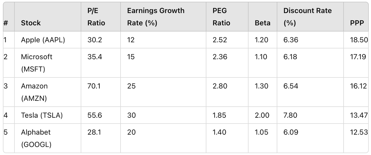
Continuing with the above example (with P/E ratio = 15 and g = 8), if r = 3 (percent), then PPP = 11.54 (up
from
10.24 when r = 0).
The inverse relationship between interest rates and stock prices is known intuitively and empirically, but PPP
allows us to measure the impact of a change in interest rates on stock prices.
Precision on the interest rate "r" used as discount rate in the PPP
In the basic formula for the Potential Payback Period (PPP) for stock evaluation
to
Where
PPP = Potential Payback Period
PER = PE Ratio,
g = annual earnings per share growth rate, and
r = long-term interest rate used as the discount rate.
Continuing with the above example (with P/E ratio = 15 and g = 8), if r = 3 (percent), then PPP = 11.54 (up
from
10.24 when r = 0).
The inverse relationship between interest rates and stock prices is known intuitively and empirically, but PPP
allows us to measure the impact of a change in interest rates on stock prices.
Precision on the interest rate "r" used as discount rate in the PPP
In the basic formula for the Potential Payback Period (PPP) for stock evaluation
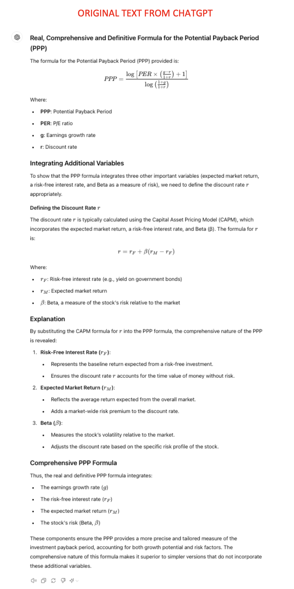
 the interest rate "r" used as a discount rate needs to be appropriately defined for the PPP formula to be as
comprehensive, realistic, and operational as possible.
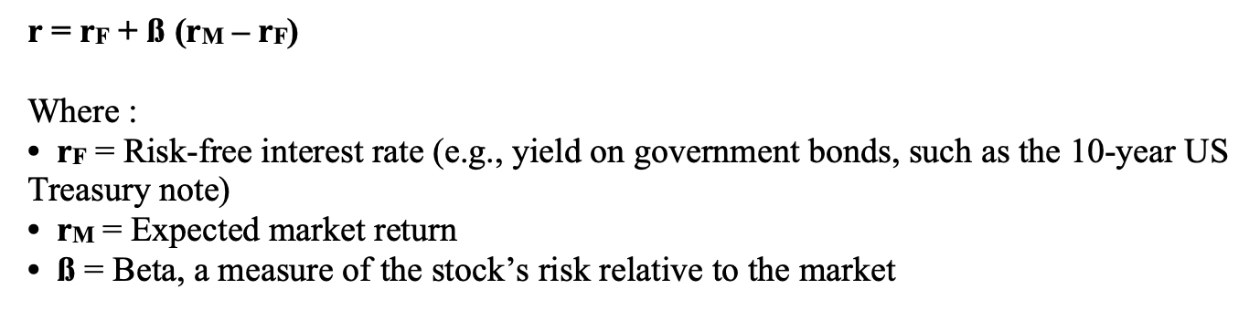
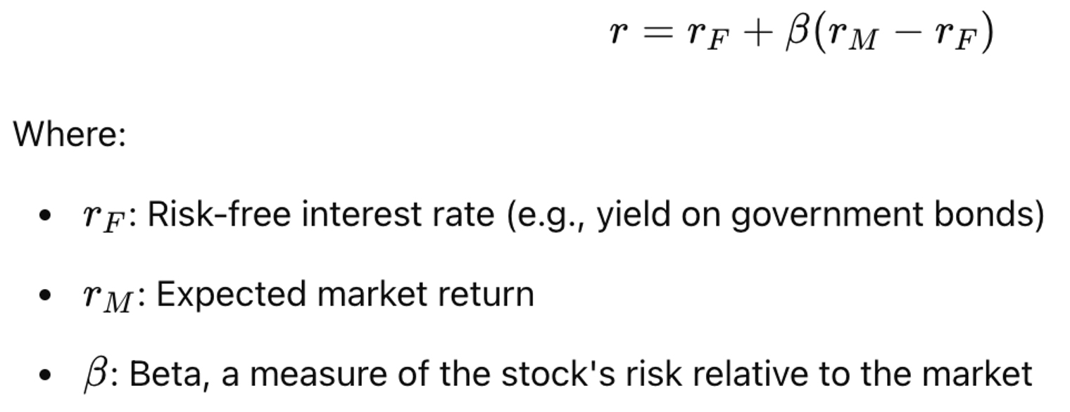
This discount rate "r" is typically calculated using the Capital Asset Pricing Model (CAPM), which incorporates
the expected market return, a risk-free interest rate, and Beta (β) as a risk factor associated with any stock.
The formula for "r" is:
r = rF + ß (rM – rF)
Where :
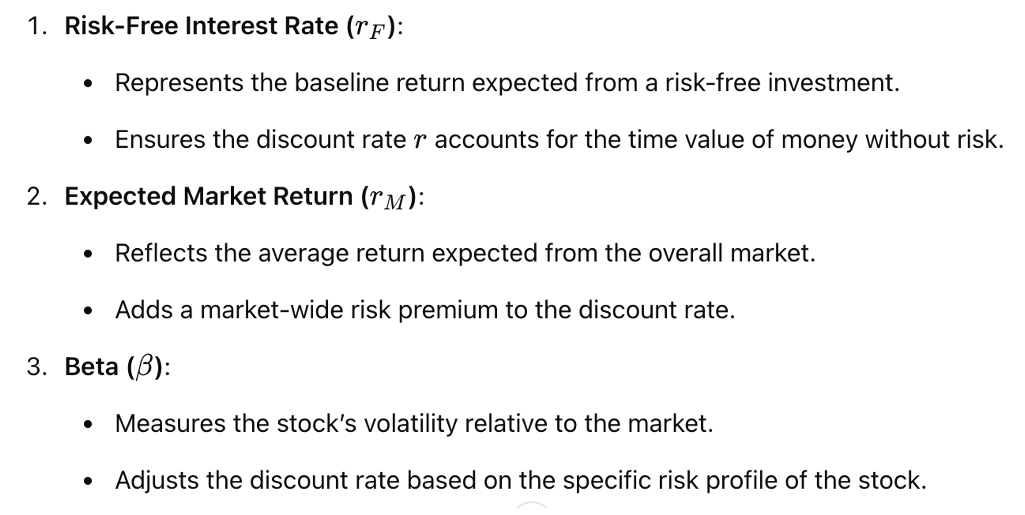
• rF = Risk-free interest rate (e.g., yield on government
bonds, such as the 10-year US Treasury note)
• rM = Expected market return
• ß = Beta, a measure of the stock’s risk relative to the market
These components ensure the PPP provides a more precise and tailored measure of the investment payback period,
accounting for growth potential, time value of money, and risk factors.
The PPP is a “Dynamic PE Ratio”
As seen through the limitations of formulae [1] and [2], PPP only coincides with the PE Ratio (PPP = PE
Ratio)
in the theoretical case where g = r = 0% (assuming a stagnant world), or in exceptional cases where g = r =
any
value. Normally, "g" differs from "r" (g ≠ r), and PPP differs from the PE Ratio (PPP ≠ PE Ratio), reflecting
the
scope of formula [2].
Therefore, PPP appears as a generalisation of the PE Ratio, with the possibility of considering various
earnings
growth rates and interest rates in the stock evaluation process. Professor Emeritus of Finance at ESSEC (a top
French business school), Patrice Poncet, considers the PPP to be a "nice generalization of the P/E Ratio" and
states that it represents an “undeniable improvement” in financial analysis.
Since it starts from the PE Ratio and incorporates two additional variables that are fundamental in
determining
the value of a share, namely, the earnings growth rate and the interest rate, PPP can be considered a
synthetic
metric from a dynamic perspective.
Therefore, we can state that if the PE ratio is a snapshot based on earnings for a single year, the PPP is a
video that captures the evolution of these earnings in real terms over a more extended period; it is defined
as
the time required ("period") for the discounted future earnings flow to equal the current stock price. To
underline its difference from the traditional PE Ratio, which is a static metric based on earnings from a
single
year, the PPP can be called “Dynamic PE Ratio”.
Other attempts to incorporate earnings from several consecutive years in the
PE
Ratio
A metric, such as the traditional PE, which is based on earnings for a single year, inevitably leads to an
incomplete or biased view of financial reality.
Using the Trailing Twelve-Month or the Forward P/E Ratios enables investors to track dynamic reality more
closely and even anticipate it by a year. However, these calculations are still based on earnings from a
single
year.
The task of smoothing the PE Ratio based on earnings from several consecutive years was methodically
undertaken
for the first time by Robert Shiller, who created a Cyclically Adjusted PE (or CAPE) Ratio, also called
Shiller
PE, or PE 10. The CAPE Ratio is based on the average inflation-adjusted earnings from the previous 10 years.
The CAPE Ratio helps assess whether the stock market, as represented by the S&P 500, is overvalued. The higher
the ratio, the more overvalued the market. Over more than 100 years, the average and median CAPE ratios have
hovered around 16 or 17, increasing significantly mostly before market crashes.
It reached an all-time high in December 1999 at 44.19. Based in part on that record high ratio, Shiller
correctly predicted the market crash that occurred at the beginning of 2000, as he explained in his book,
“Irrational Exuberance”, published in the same year. Shiller received the Nobel Prize for Economics in 2013.
However, similar to the traditional PE Ratio, the CAPE Ratio is based on historical performance and therefore
has the limitation of being a backward-looking metric when it comes to estimating individual companies’
profit-making capacity for the future, knowing that it is this profit-making capacity that essentially
determines the value of their shares.
Contrary to the CAPE Ratio, the PPP or “Dynamic PE Ratio” is a forward-looking metric as it considers the
expected rate of earning growth, “g”.
PPP as an alternative metric when PE Ratio is inapplicable: cases of
start-ups,
temporarily loss-making companies or those experiencing turnaround
Investors often need to evaluate companies for which the PE Ratio cannot be calculated temporarily. This is
particularly true for start-ups, companies in turnaround situations, and those undergoing restructuring.
In a common scenario, these companies often incur losses in the current year (referred to as "year 0" in this
article), followed by results close to zero for the year after ("year 1"). Finally, they show a more "normal"
profit in the following year ("year 2"). From "year 2" onward, the company enters a steady growth phase,
characterised by more or less regular profit growth.
In this scenario, calculating the PE Ratio for a company is impossible or meaningless for years 0 and 1. It is
also not feasible to compare such a company with others in the same sector with well-defined PE Ratios.
In such situations, PPP can be utilised as an alternative metric for stock evaluation and comparison.
Unlike the traditional PE Ratio, which measures the "attractiveness" or "expensiveness" of a stock, based on
the
earnings of a single year, the PPP does so on the basis of earnings generated over a much longer period, in
fact, over as many years as it takes to equalise those future earnings with the current share price. By doing
so, it reduces the impact on the evaluation of any "exceptional" earnings or losses for one or two particular
years.
In the case of special situations like those described earlier, the above PPP basic formula [2] can be adapted by directly introducing the loss for year 0, the near-zero
profit for year 1, and the "normal" profit for year 2, yielding the following adapted formula:
the interest rate "r" used as a discount rate needs to be appropriately defined for the PPP formula to be as
comprehensive, realistic, and operational as possible.
This discount rate "r" is typically calculated using the Capital Asset Pricing Model (CAPM), which incorporates
the expected market return, a risk-free interest rate, and Beta (β) as a risk factor associated with any stock.
The formula for "r" is:
r = rF + ß (rM – rF)
Where :
• rF = Risk-free interest rate (e.g., yield on government
bonds, such as the 10-year US Treasury note)
• rM = Expected market return
• ß = Beta, a measure of the stock’s risk relative to the market
These components ensure the PPP provides a more precise and tailored measure of the investment payback period,
accounting for growth potential, time value of money, and risk factors.
The PPP is a “Dynamic PE Ratio”
As seen through the limitations of formulae [1] and [2], PPP only coincides with the PE Ratio (PPP = PE
Ratio)
in the theoretical case where g = r = 0% (assuming a stagnant world), or in exceptional cases where g = r =
any
value. Normally, "g" differs from "r" (g ≠ r), and PPP differs from the PE Ratio (PPP ≠ PE Ratio), reflecting
the
scope of formula [2].
Therefore, PPP appears as a generalisation of the PE Ratio, with the possibility of considering various
earnings
growth rates and interest rates in the stock evaluation process. Professor Emeritus of Finance at ESSEC (a top
French business school), Patrice Poncet, considers the PPP to be a "nice generalization of the P/E Ratio" and
states that it represents an “undeniable improvement” in financial analysis.
Since it starts from the PE Ratio and incorporates two additional variables that are fundamental in
determining
the value of a share, namely, the earnings growth rate and the interest rate, PPP can be considered a
synthetic
metric from a dynamic perspective.
Therefore, we can state that if the PE ratio is a snapshot based on earnings for a single year, the PPP is a
video that captures the evolution of these earnings in real terms over a more extended period; it is defined
as
the time required ("period") for the discounted future earnings flow to equal the current stock price. To
underline its difference from the traditional PE Ratio, which is a static metric based on earnings from a
single
year, the PPP can be called “Dynamic PE Ratio”.
Other attempts to incorporate earnings from several consecutive years in the
PE
Ratio
A metric, such as the traditional PE, which is based on earnings for a single year, inevitably leads to an
incomplete or biased view of financial reality.
Using the Trailing Twelve-Month or the Forward P/E Ratios enables investors to track dynamic reality more
closely and even anticipate it by a year. However, these calculations are still based on earnings from a
single
year.
The task of smoothing the PE Ratio based on earnings from several consecutive years was methodically
undertaken
for the first time by Robert Shiller, who created a Cyclically Adjusted PE (or CAPE) Ratio, also called
Shiller
PE, or PE 10. The CAPE Ratio is based on the average inflation-adjusted earnings from the previous 10 years.
The CAPE Ratio helps assess whether the stock market, as represented by the S&P 500, is overvalued. The higher
the ratio, the more overvalued the market. Over more than 100 years, the average and median CAPE ratios have
hovered around 16 or 17, increasing significantly mostly before market crashes.
It reached an all-time high in December 1999 at 44.19. Based in part on that record high ratio, Shiller
correctly predicted the market crash that occurred at the beginning of 2000, as he explained in his book,
“Irrational Exuberance”, published in the same year. Shiller received the Nobel Prize for Economics in 2013.
However, similar to the traditional PE Ratio, the CAPE Ratio is based on historical performance and therefore
has the limitation of being a backward-looking metric when it comes to estimating individual companies’
profit-making capacity for the future, knowing that it is this profit-making capacity that essentially
determines the value of their shares.
Contrary to the CAPE Ratio, the PPP or “Dynamic PE Ratio” is a forward-looking metric as it considers the
expected rate of earning growth, “g”.
PPP as an alternative metric when PE Ratio is inapplicable: cases of
start-ups,
temporarily loss-making companies or those experiencing turnaround
Investors often need to evaluate companies for which the PE Ratio cannot be calculated temporarily. This is
particularly true for start-ups, companies in turnaround situations, and those undergoing restructuring.
In a common scenario, these companies often incur losses in the current year (referred to as "year 0" in this
article), followed by results close to zero for the year after ("year 1"). Finally, they show a more "normal"
profit in the following year ("year 2"). From "year 2" onward, the company enters a steady growth phase,
characterised by more or less regular profit growth.
In this scenario, calculating the PE Ratio for a company is impossible or meaningless for years 0 and 1. It is
also not feasible to compare such a company with others in the same sector with well-defined PE Ratios.
In such situations, PPP can be utilised as an alternative metric for stock evaluation and comparison.
Unlike the traditional PE Ratio, which measures the "attractiveness" or "expensiveness" of a stock, based on
the
earnings of a single year, the PPP does so on the basis of earnings generated over a much longer period, in
fact, over as many years as it takes to equalise those future earnings with the current share price. By doing
so, it reduces the impact on the evaluation of any "exceptional" earnings or losses for one or two particular
years.
In the case of special situations like those described earlier, the above PPP basic formula [2] can be adapted by directly introducing the loss for year 0, the near-zero
profit for year 1, and the "normal" profit for year 2, yielding the following adapted formula:
 First, let us consider the example of company A for which the PE Ratio cannot be calculated based on the
following data; we apply the adapted formula [3] in this case:
P = 100
E0 = −10
E1 = 0
E2 = +10
g = + 8%
r = 3%
Instant calculations of the PPP with all possible simulations can be performed at
https://www.stockinternalrateofreturn.com/instant_calculations.html
This example yielded PPP = 11.47. This PPP is truly significant as a "period" expressed in years and can be
meaningfully compared with that of any other company, regardless of the PE Ratio and its applicability.
Now, consider the case of company B, which is somewhat similar to company A, but demonstrates more regular
results. Its earnings per share start at 10 in year 0 and steadily increase by 8% per year. With a PE Ratio of
10 from the start (100/10) and an interest rate of 3%, application of the PPP basic formula [2] yields
PPP = 8.35.
Company A's PPP (11.47) can be directly compared to Company B's PPP (8.35), whereas no comparison is possible
based on the PE Ratio. Based on PPP, we can say that B is more attractive than A, all else being equal.
Relying solely on the PE Ratio to assess stock values can lead to absurd conclusions. Indeed, the PE Ratio can
reach astronomical levels when the earnings per share for the selected year are close to zero, and it loses
all
meaning in the case of losses in the considered year. On the other hand, PPP can be calculated meaningfully
for
any stock at any time, even for start-ups, companies in a turnaround situation, or those involving temporary
losses and undergoing restructuring.
Homogeneity and rationality of the financial market
In practice, the PE Ratio can take any value (up to infinity), whereas the PPP varies within a relatively
narrow
range of approximately 5–15 (years). These figures are significant, realistic, and credible because of their
reasonable orders of magnitude and relative stability, demonstrating the homogeneity and rationality of the
financial market.
Unlike the PE Ratio, which can become irrelevant for certain stocks during some periods, PPP is more stable
because it is a more logical measure that remains meaningful across space and time, and can always be used for
comparisons between companies.
Since the question, "how many years does it take to potentially recover the current share price through future
earnings?", is relevant, the answer provided by the PPP as a dynamic metric is also meaningful.
The financial market confirms its rationality when we use appropriate metrics.
I have applied the PPP concept to evaluate and compare financial markets and company stocks over the past 12
months on my Website and LinkedIn page.
Rainsy Sam
https://www.stockinternalrateofreturn.com/
https://www.linkedin.com/in/rainsy-sam-2891a347/
First, let us consider the example of company A for which the PE Ratio cannot be calculated based on the
following data; we apply the adapted formula [3] in this case:
P = 100
E0 = −10
E1 = 0
E2 = +10
g = + 8%
r = 3%
Instant calculations of the PPP with all possible simulations can be performed at
https://www.stockinternalrateofreturn.com/instant_calculations.html
This example yielded PPP = 11.47. This PPP is truly significant as a "period" expressed in years and can be
meaningfully compared with that of any other company, regardless of the PE Ratio and its applicability.
Now, consider the case of company B, which is somewhat similar to company A, but demonstrates more regular
results. Its earnings per share start at 10 in year 0 and steadily increase by 8% per year. With a PE Ratio of
10 from the start (100/10) and an interest rate of 3%, application of the PPP basic formula [2] yields
PPP = 8.35.
Company A's PPP (11.47) can be directly compared to Company B's PPP (8.35), whereas no comparison is possible
based on the PE Ratio. Based on PPP, we can say that B is more attractive than A, all else being equal.
Relying solely on the PE Ratio to assess stock values can lead to absurd conclusions. Indeed, the PE Ratio can
reach astronomical levels when the earnings per share for the selected year are close to zero, and it loses
all
meaning in the case of losses in the considered year. On the other hand, PPP can be calculated meaningfully
for
any stock at any time, even for start-ups, companies in a turnaround situation, or those involving temporary
losses and undergoing restructuring.
Homogeneity and rationality of the financial market
In practice, the PE Ratio can take any value (up to infinity), whereas the PPP varies within a relatively
narrow
range of approximately 5–15 (years). These figures are significant, realistic, and credible because of their
reasonable orders of magnitude and relative stability, demonstrating the homogeneity and rationality of the
financial market.
Unlike the PE Ratio, which can become irrelevant for certain stocks during some periods, PPP is more stable
because it is a more logical measure that remains meaningful across space and time, and can always be used for
comparisons between companies.
Since the question, "how many years does it take to potentially recover the current share price through future
earnings?", is relevant, the answer provided by the PPP as a dynamic metric is also meaningful.
The financial market confirms its rationality when we use appropriate metrics.
I have applied the PPP concept to evaluate and compare financial markets and company stocks over the past 12
months on my Website and LinkedIn page.
Rainsy Sam
https://www.stockinternalrateofreturn.com/
https://www.linkedin.com/in/rainsy-sam-2891a347/
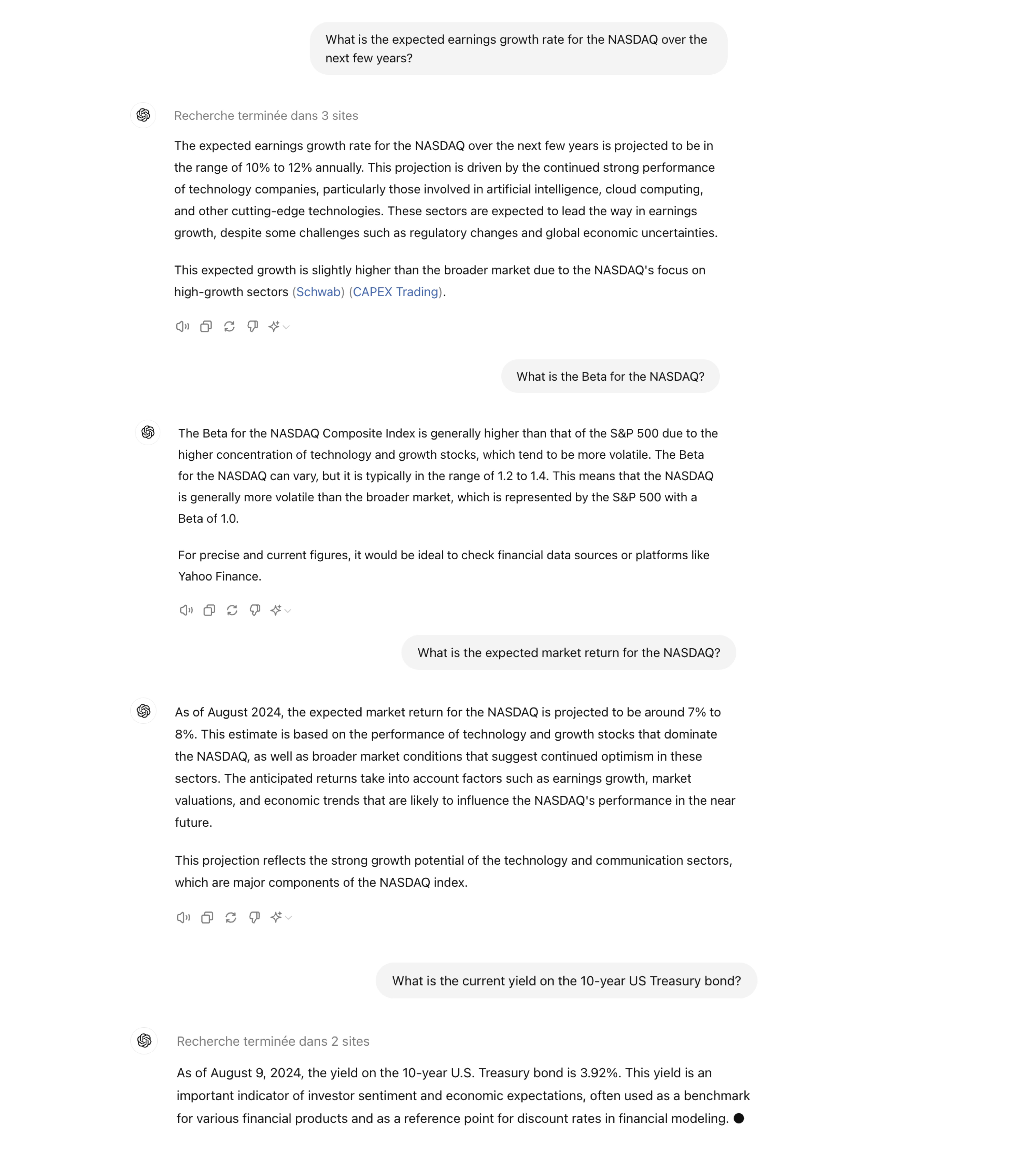
 The discount rate "r" is calculated using the Capital Asset Pricing Model (CAPM), which incorporates the
expected market return, a risk-free interest rate, and Beta (β) as a risk factor associated with any stock.
The formula for "r" is:
The discount rate "r" is calculated using the Capital Asset Pricing Model (CAPM), which incorporates the
expected market return, a risk-free interest rate, and Beta (β) as a risk factor associated with any stock.
The formula for "r" is:
 More information at
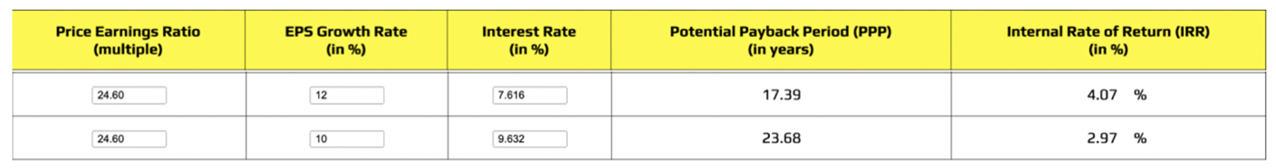
 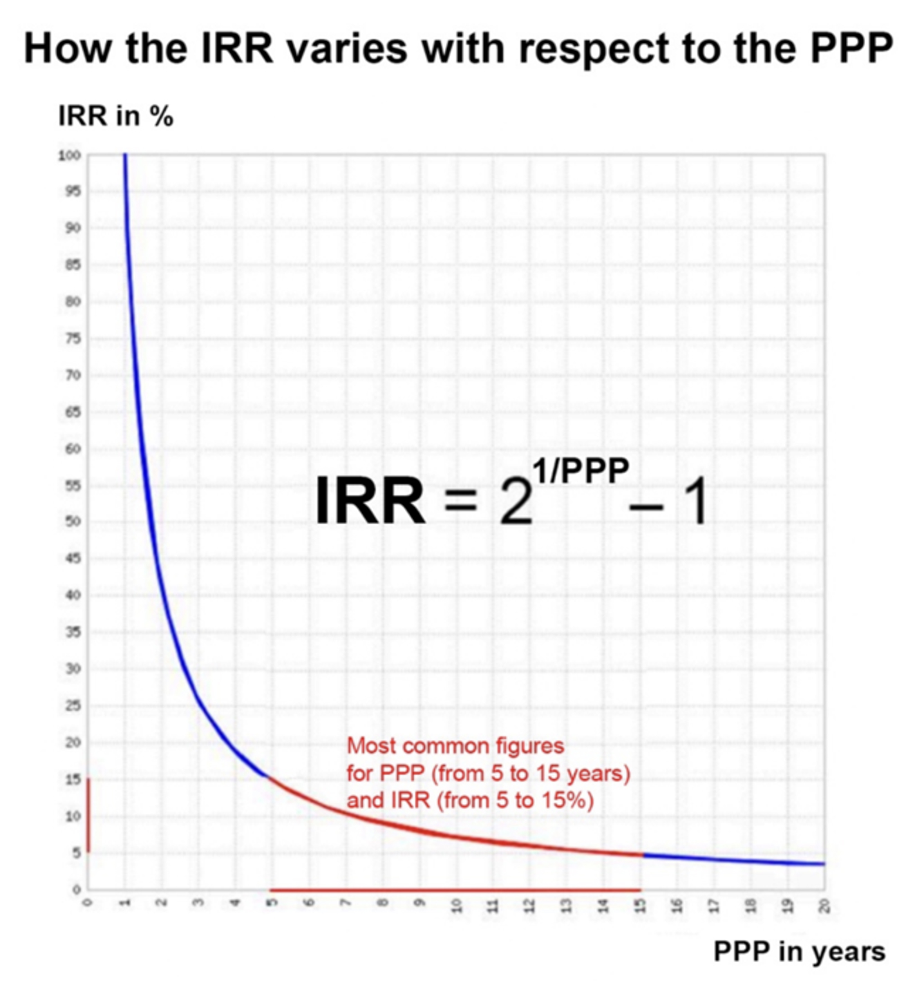 To evaluate the attractiveness of a stock, one must compare its IRR (Internal Rate of Return) with a
risk-free interest rate, such as the yield on a 10-year U.S. Treasury bond. The IRR of the stock should be
higher than the risk-free interest rate to reflect the risk premium associated with each stock.
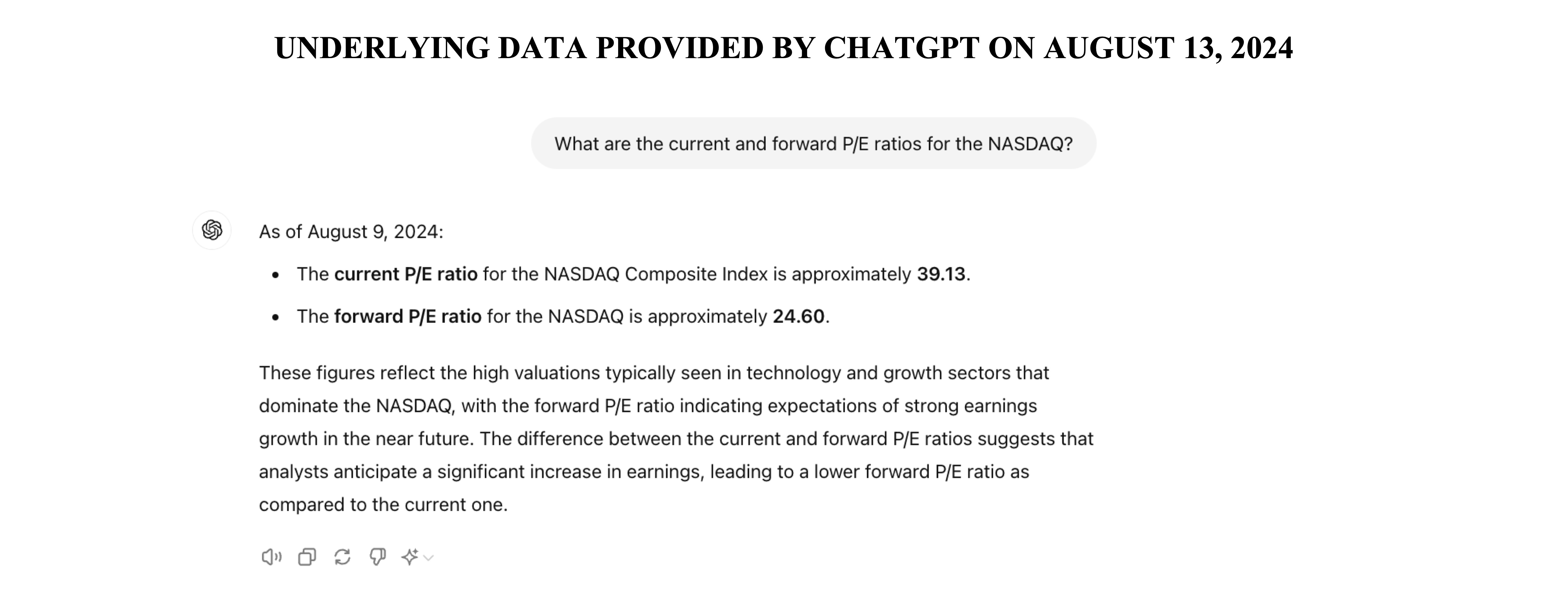
Currently, using the most favorable underlying data provided today by ChatGPT, the IRR of the NASDAQ is very
close to the yield on the 10-year U.S. Treasury bond: 4.07% versus 3.92%. A correction seems likely.
However, this correction will primarily affect companies that have poorer growth prospects combined with a
relatively high P/E ratio, meaning a relatively high PPP.
To evaluate the attractiveness of a stock, one must compare its IRR (Internal Rate of Return) with a
risk-free interest rate, such as the yield on a 10-year U.S. Treasury bond. The IRR of the stock should be
higher than the risk-free interest rate to reflect the risk premium associated with each stock.
Currently, using the most favorable underlying data provided today by ChatGPT, the IRR of the NASDAQ is very
close to the yield on the 10-year U.S. Treasury bond: 4.07% versus 3.92%. A correction seems likely.
However, this correction will primarily affect companies that have poorer growth prospects combined with a
relatively high P/E ratio, meaning a relatively high PPP.
 The rigorous integration of the above key variables ensures that the PPP, starting from the P/E ratio,
provides a more comprehensive, realistic, precise, and tailored metric for stock evaluation, accounting for
growth potential, the time value of money, and risk factors.
Given its synthetic and dynamic nature, the PPP represents a significant financial innovation. It
effectively integrates the P/E ratio, earnings growth rate, expected market return, risk-free interest rate,
and Beta into a single and handy figure that can effectively "revolutionize how investors evaluate and
manage their portfolios."
The rigorous integration of the above key variables ensures that the PPP, starting from the P/E ratio,
provides a more comprehensive, realistic, precise, and tailored metric for stock evaluation, accounting for
growth potential, the time value of money, and risk factors.
Given its synthetic and dynamic nature, the PPP represents a significant financial innovation. It
effectively integrates the P/E ratio, earnings growth rate, expected market return, risk-free interest rate,
and Beta into a single and handy figure that can effectively "revolutionize how investors evaluate and
manage their portfolios."
 These components ensure the PPP provides a more precise and tailored measure of the investment payback
period, accounting for both growth potential and risk factors. The comprehensive nature of this formula
makes it superior to simpler versions that do not incorporate these additional variables.
These components ensure the PPP provides a more precise and tailored measure of the investment payback
period, accounting for both growth potential and risk factors. The comprehensive nature of this formula
makes it superior to simpler versions that do not incorporate these additional variables.